Natural terrains modeling

This study is performed in the frame of a contract with Dassault Aviation.
The problem posed by Dassault Aviation is that of digital terrains assessment. Typically, several sets of digital data are available for a single region. They originate from different modalities (e.g. radar images, geographical data . . .), have different resolutions, contain errors, and are locally incomplete. The challenge is to merge these data so as to obtain both a more reliable description and a “grade” for each point, i.e. a number assessing the confidence one has in this particular value.

Our strategy is to model terrains with well-chosen stochastic processes, to estimate the parameters of the models, and then to use standard tools from statistics to qualify each point.
A first possibility is to use mBm, which was precisely invented with this application in mind. More recently, we have used the SRMP as an alternative and sometimes more adapted model. Results using this last approach mainly show two facts:

• on small enough zones, natural terrains do indeed exhibit a measurable relation between altitude and regularity, so that a modelling with a self-regulating process makes sense,
• estimation of the g function of the SRMP indicates that young mountains (such as Himalaya and the Rocky Mountains) behave differently from older ones (such as Tibesti and Massif Central): for young mountains, points at higher altitudes are more irregular. The reverse seems to be true for old mountains, possibly due to erosion phenomena (see figure below).

Our current work focuses on:

1. the search for better estimation methods of the parameters of the mBm modelling the terrains,
2. a more thorough exploration of the relevance of SRP for terrain modelling, along with robust estimation methods,
3. the development of an interpolation method based on local regularity, allowing to assess the quality of the available data.

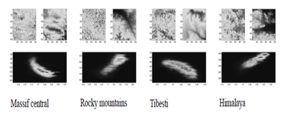
In each cell, the upper-right figure is the original image of size 512x512 pixels. The upper-left figure displays the exponent at each point of the image and the lower figure shows the density of the scatter plot in the “altitude-exponent” plane.